The Binomial Distribution
Bridging the gap from description to inference
I recently had a conversation on Mastodon about how someone never understood the binomial distribution when they took a statistics class that had a terrible teacher (who apparently played the lottery despite teaching statistics), which is a shame because it really is an important thing and I think, if well explained, not actually that difficult.
It also looks pretty.
But let’s rewind a bit. We’ll get back to the pretty graph, I promise.
Why is it important?
An entry-level class in statistics will mostly cover what’s called descriptive statistics. The goal is, as the name says, to describe things as they are. The bread and butter here are means, variances, medians, quantiles, and several other values that can describe a sample of data. The crucial detail is that the sample is what’s described, not the real world.
If you measure the height of 100 trees, you can say what the average height among those 100 trees is, but you can’t say what the average height of all trees is.
There’s usually also some probability math in those classes, answering questions like “What’s the probability of getting all heads on 5 coin flips?” (It’s 3.12% assuming the coin is fair).
And then there’s inference statistics, where we use sampled data to make inferences or predictions about things that are not in the sample. This is where hypotheses are tested, models are built, tests are done, and p-values are everywhere. In my experience tutoring a lot of students through it, this is also where a lot of them get lost. Somewhere between these areas of statistics they miss a crucial thing, a thing that bridges those two worlds.
That bridge is the binomial distribution.
What is it used for?
Let’s say you and a friend play a round of heads or tails every time you have conflicting options on something and have to come to a decision. You’re not really a cash person so it’s usually your friend pulling out a coin and flipping it. They always pick heads.
After a while you get the feeling that something is off, and you keep track of the results. over the last 50 coin flips your friend won 32` times. Now that’s not impossible, but it’s also pretty far off from the 50% you’d expect. So how unlikely is this result?
This is a question that one of the simplest statistical tests can answer: the binomial test.
    Exact binomial test

data:  k and n
number of successes = 32, number of trials = 50, p-value = 0.03245
alternative hypothesis: true probability of success is greater than 0.5
95 percent confidence interval:
 0.5142308 1.0000000
sample estimates:
probability of success
                  0.64
This is the output of the test when done in R, a popular statistics programming language, but I’m not here to talk about R. The interesting part is the p-value of 0.03245 or roughly 3.24%.
A p-value in a statistical test usually tells you the probability of getting the sample you actually have, or an even more extreme one, given that the null hypothesis is true. The null hypothesis is assuming that whatever we’re looking at is not different from the the overall population it came from. In this case we assume that your friend’s coin is just like the vast majority of coins out there and that it makes for a fair 50/50 coin flip.
So, this binomial test answers the question “Assuming the coin has a 50% chance to show heads, how likely is it to get 32 heads out of 50 flips?”.
A 3.24% probability that this is actually a fair coin is not much. It is in fact under the 5% threshold for p-values used in many scientific papers. It would be absolutely valid to reject the null-hypothesis assumption here and have a talk with your friend about their weirdly “lucky” coin.
But how did the test get from “32 out of 50” to those 3.24%?
How to build it
Let’s start with one coin flip. With a fair coin the probability to win is 50%, that’s what it means for the coin to be fair. What about two coin flips? Assuming we pick heads, how probable is it to win at least once?
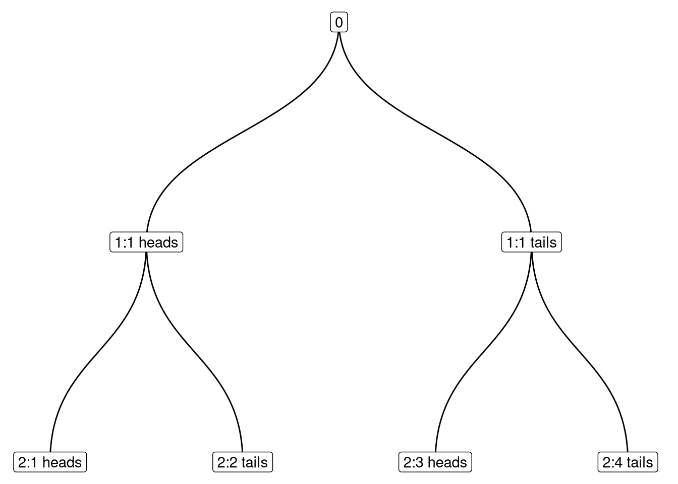
We can see there’s 3 paths here that contain at least one win:
- heads \(\rightarrow\) tails
- tails \(\rightarrow\) heads
- heads \(\rightarrow\) heads
So, 3 out of 4 possible flips will give you at least one win: \(\frac{3}{4} = 75\%\). For a small number of flips, and a fair 50/50 coin, this is still pretty easy to keep track of and calculate but it gets overwhelming very quickly. What’s the probability of getting at least 11 heads out of 15 flips? Good luck doing that manually.
I actually skipped a step there because in this small example it easier that way. In order to arrive at those \(75\%\), we could also ask: “Out of the 4 possible sequences of 2 flips, how many have exactly one win, and how many have two wins. The answer is 2 and 1 respectively. Since we were looking for any sequence with at least one win, so either 1 or 2, we add those up and get the 3 out of 4 flips.
This is how it will work for bigger examples. We figure out how many possible flip sequences there are in total, and then how many have as many wins as we’re interested in, then how many have one more, and one more, all the way up to the one that’s all wins. For our “11 out of 15” example that means:
| wins | sequences |
|---|---|
| 11 | 1365 |
| 12 | 455 |
| 13 | 105 |
| 14 | 15 |
| 15 | 1 |
Summing those up we get 1,941 out of a total of 32,768 possible sequences of 15 flips, a probability of 5.92%.
Putting in the engine: the binomial coefficient
As you probably noticed I skipped over something there again. How did I get all those numbers of how many sequences with whatever many wins there are? I used the binomial coefficient:
\[\binom{n}{k} = \frac{n!}{k!*(n-k)!}\]
Don’t let that fancy equation intimidate you, we’ll pick it apart. What’s important here is that \(\binom{n}{k}\) is called the binomial coefficient, it’s been known to humans in some form for hundreds of years, and it answers this question:
“In how many different ways can I pull \(k\) items out of a pool of \(n\) items, if I put them back in every time?”
Or rephrased for our coin flip example:
If I flip a coin 15 times, in how many different ways could 11 wins appear?
BTW: If you’re wondering what that “\(!\)” in the equation is, that’s called a factorial. It works like this:
\[5! = 5 * 4 * 3 * 2 *1 = 120\]
It’s the number of possible arrangements of a number of items in a row. If you put 5 books on a shelf, there’s 120 possible orders to put them in. There’s an intuitive way to look at this too: You can place the first book in any of the five total spots. Afterwards the second book only has four free spots available, the third book has three, the fourth book only goes in one of two free spots, and then there’s one spot left for the fifth book.
The formula for the binomial coefficient makes use of these multiple times:
\(n!\) gives us the number of total possible arrangements of all the coin flips. This will often be a very large number.
\(k!\) is the number of total possible arrangements of the winning flips.
\((n-k)!\) is the number of arrangement s of all the remaining flips.
We divide the total number of arrangements by the product of the other two since all wins are identical to us, as are all losses. If we win two flips in a row, it doesn’t matter if those two switch places. They are indistinguishable and independent from each other. The two factorials in the denominator take care of removing all those outcomes that are duplicates because they have the same sequence of winning and losing.
Let’s check out what a plot of the binomial coefficient looks like:
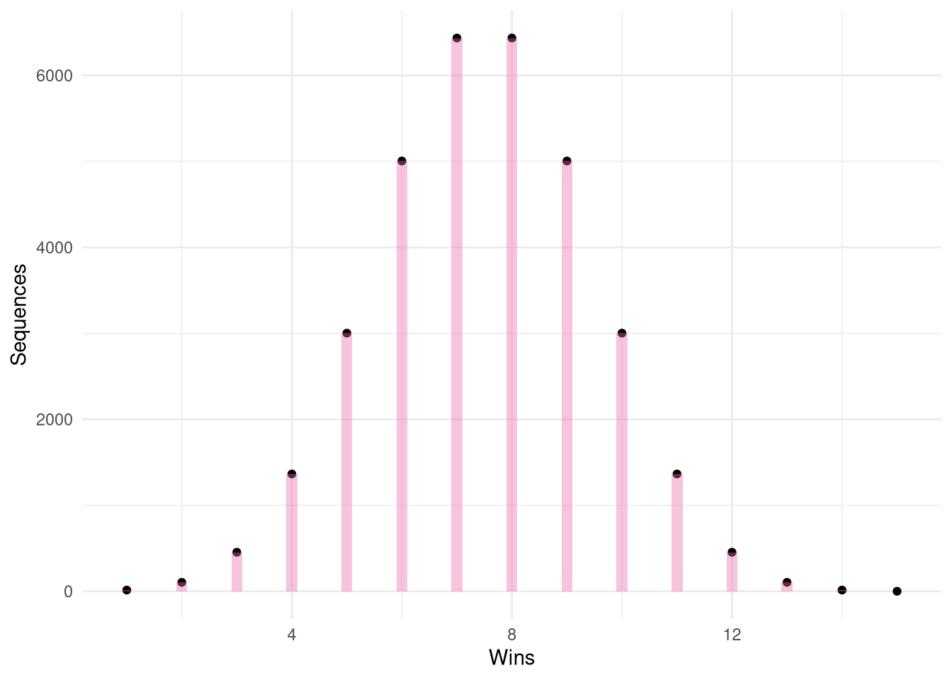
That looks somewhat familiar, doesn’t it? And it should make intuitively sense too. How many ways can you win once of 15 coin flips? 15, because you could win on the 1st attempt, the 2nd, 3rd, etc. And how many different ways could you win 15 times? Exactly one, because you’d have to win every time. This is why the left and right end of the graph are very low. The middle range is where most of the possible combinations are.
But we’re not there yet. This is a plot of how many possible ways you could pull a number of items from a pool, not of probability. And so far we haven’t considered the option that the coin might not be entirely fair either.
Assembling it all
So far we have \(\binom{n}{k}\) which gives us the total number of the outcomes we’re interested in, like every row of 15 coin flips with exactly 11 wins.
We need to add information about how probable each of those outcomes is. In the case of a fair coin, this is just \(0.5^n\) because each flip has a 50% (0.5) probability to win or lose, and the total probability of several things happening together, 15 flips each with a specific outcome here, is the product of all those individual probabilities, so \(0.5 * 0.5 * 0.5 \dots\) which can be shortened to \(0.5^n\). It’s \(0.5^{15}\) in our case, which is a tiny number but that’s OK since there are also a lot of possible sequences of flips.
So for the fair coin flip we multiply the probability of one specific sequence with the number of possible sequences:
\[Pr(k,n) = \binom{n}{k} * p^n\]
\(Pr(k,n)\) here is the probability of getting exactly \(k\) wins out of \(n\) fair coin flips, \(p\) being the probability of winning a single flip so \(0.5\). Plotting it looks like this:
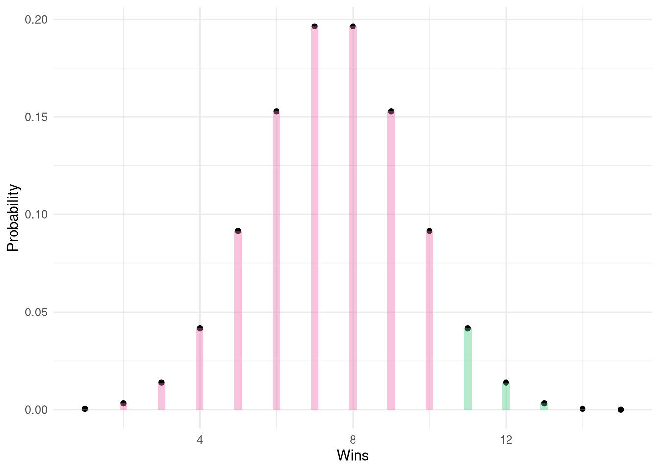
This is expected, getting 11 or more wins (the green bars) out of 15 flips is pretty unlikely.
To finish it, we need to add a way to represent an unfair coin, or more generally any random event with two possible outcomes and constant but not necessarily equal probabilities.
Instead of \(n\) identical events, we’re looking for \(k\) wins and \(n-k\) losses, where the probability for winning is \(p\) and the probability for losing is \(1-p\) because there are just two outcomes and they have to add up to \(1.0\) or \(100\%\).
So the probability for each sequence of flips is the probability of winning raised to the power of the number of wins (instead of all flips) and the probability of losing raised to the power of the number of losses because both the wins and the losses have to happen in order to produce that particular sequence. And then just as before is gets multiplied by the number of sequences that have that amount of wins and losses, given by the binomial coefficient. Finally, we get the real formula for the binomial distribution, the pure undiluted stuff:
\[ Pr(k) = \binom{n}{k} * p^k * (1-p)^{n-k}\]
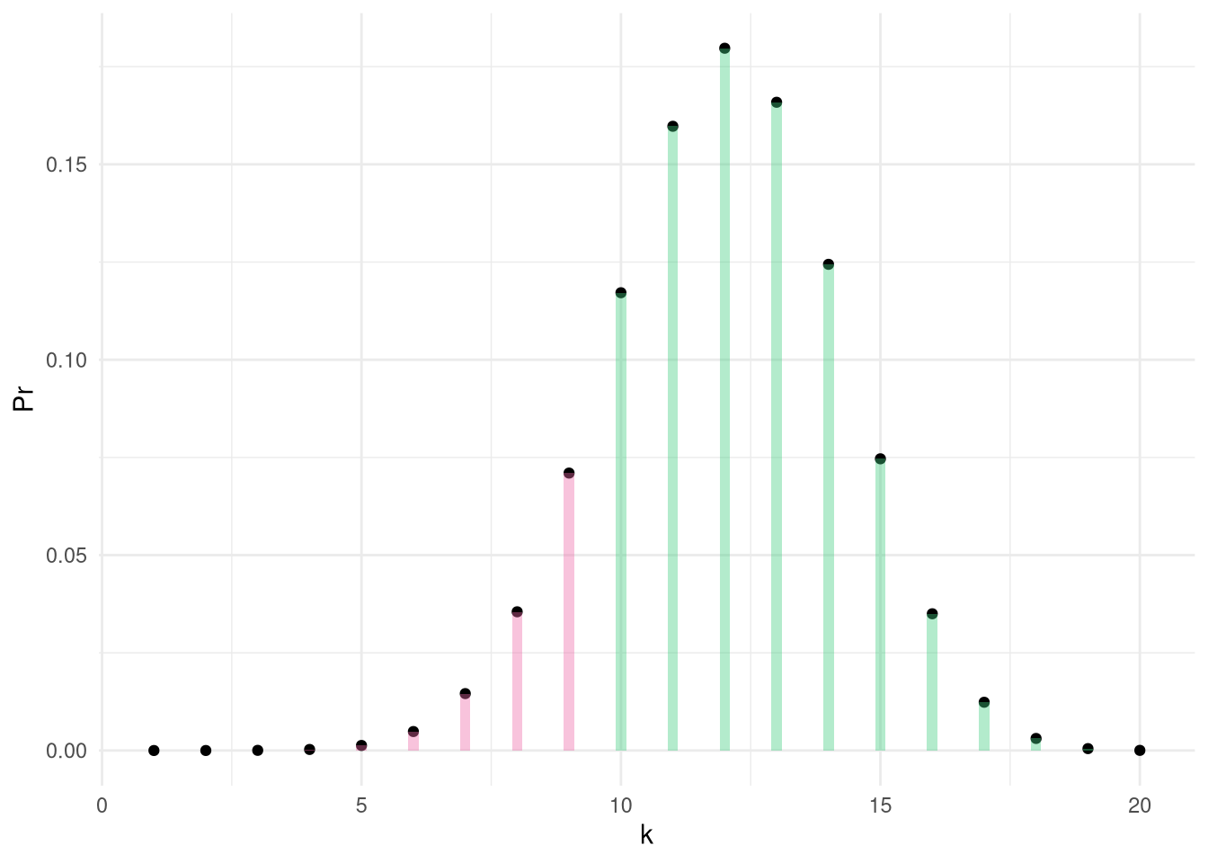
Now we can examine unfair coins and return to the example we started with where your friend won 32 out of 50 flips. Here’s the plot for that assuming a fair coin:
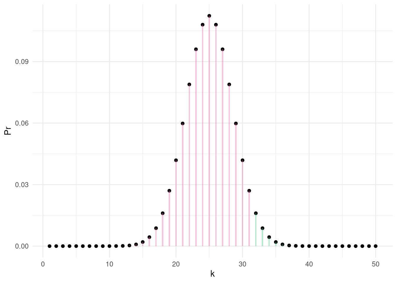
This tiny green portion just illustrates the p-value of 3.24% we got from that binomial test. That test also told us the the estimated true probability for that coin was 64%. This is the plot for that probability:
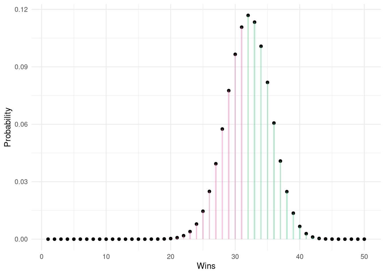
Yeah, that’s seems to line up much better with our observations.
Finishing up
In order to get a direct visual answer to the question “How probable is it to get 32 wins out of 50 flips with a 64% coin?”, we can use an alternative way of plotting this graph, as a cumulative function:
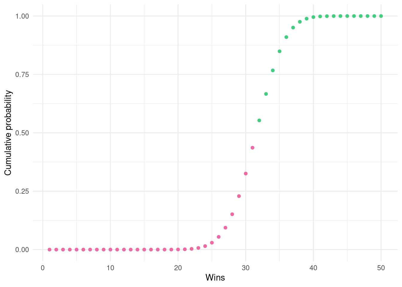
Here each point represents the probability of getting up to a certain number of wins, instead of just one specific number of wins. It also makes it very easy to see how the quickly the probabilities change in the middle section while pretty much approaching 0 or 100% at the outer parts.
Last words
The binomial distribution sits right between the world of the individual probabilities we started with where you think about single events or maybe a few of them, and the world of statistical inference where you’re much more interested in thinking about what underlying rules could explain certain observations, like how we figured out that the observation of all those coin flips an be explained by an unfair coin. We made an inference about the real world based on a limited sample of data.
The binomial distribution is a probability mass function, meaning that each point on the graph represents an actual probability for an outcome. This is a major difference from most other probability distributions that are used in statistical inference. Those are mostly probability density functions where a probability is an area under the the curve instead of a point. Another reason why it’s a bit of a bridge between the world of discrete values and events and mostly contiguous spectra of values.
That larger world is quite a wall the many beginning statistics students run into but I think, if you understand this bridge that is the binomial distribution, a lot of the things that come later will become much easier.